How does Carmaker estimates longitudinal load transfer in each tire?

[Gytakemoto]

Hi.

I was trying to model longitudinal load transfers through mechanical equations and compare it with the values measured by Carmaker.

My goal is to determine the total load of each rear tire, specially during straight acceleration runs, but preferably in any condition.

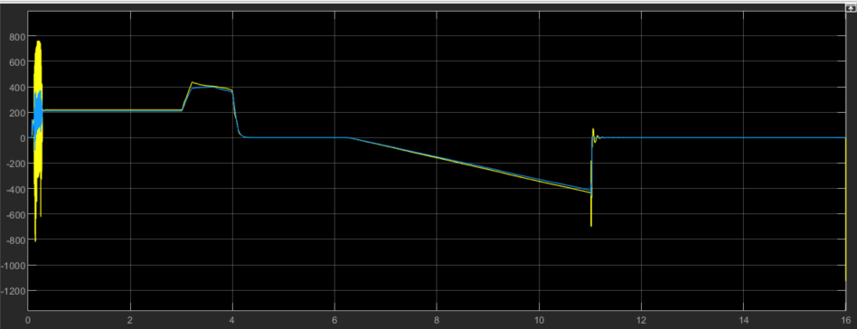
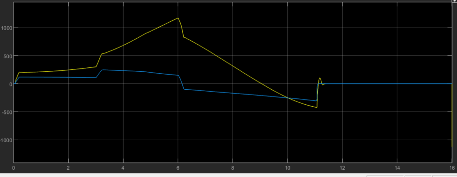
Comparing my results (exporting it from simulink to IPGControl) with Car.FzRL and Car.FzRR I noticed they are a little different, that’s why I’d like to know how does CM estimate it. It can be seem in the following figure:

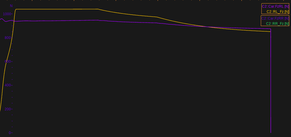
Notice I’m not only considering the longitudinal load transfers in the RL_Fz and RR_Fz, but also lateral, static and aerodynamic loads.

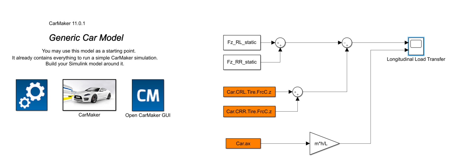
I am using the following equation to longitudinal load transfer:

\Delta W_r = \frac{h}{2L} W a_x

Where:
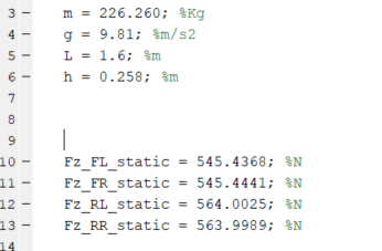
h = height of center of gravity (m)
L = wheelbase (m)
a_x = longitudinal acceleration (m/s²)
W = car weight (kg)

The rest of the equations can be seem in this document.

I suppose CM uses much more complex set of equations, but I haven’t had luck searching for better options. Other reason I can think of is that my tire model is pretty unrealistic right now, but that’s something I’m still working on.

One last hypothesis is that maybe there are some parameters in my vehicle file that’s not compatible with the values I am using on my Simulink model, but I’m also working on it and I’ve checked it multiple times.

Anyways, any help would be appreciated! I am really stuck on this problem.

[mariano.carpinelli]

Hi there,

thanks for the interesting question.

The longitudinal load transfer formula that you want to use requires an accurate knowledge of the parameters h and L, however both of them vary during a dynamic event such as a straight acceleration test.

These changes are influenced by several factors, such as the pitch center position of the front and rear suspensions, spring stiffness, changes in wheelbase due to the supension kinematics, tire vertical deflections, how the driving torque is applied to the driving wheels (e.g. inboard or outboard electric motors), etc.

As you were mentioning, all these effects are taken into account when you run a CM simulation, so if you are using constant values for h and L it is very likely that you’ll get discrepancies when you compare to CM. This gets even more involved if you are considering lateral accelerations or aero forces.

To give you a practical example I have picked up the FSE_AllWheelDrive model in the FS package and disabled the aero forces/moments, increased the spring stiffness, used very stiff tires with minimal rolling resistance and used inboard electric motors (example.zip (13.4 KB)). All these changes are meant to minimize the pitch and heave variations during an acceleration test.

I’ve then run an Equilibrium ModelCheck to determine h, L and the static weight distribution and defined these variables in Matlab:

I’ve then run an acceleration/braking test in CM for Simulink where I have implemented the Longitudinal Load Transfer formula:

As you can see in the Longitudinal Load Transfer scope the actual value (yellow line) is very close to the predicted one (blue line) obtained using the simple LLT formula where h and L are considered as constants:

However if you use the original FSE_AllWheelDrive model the assumption of h and L being constant loses its validity, see body pitch angle and body heave movements in the graph below where the green curve is the modified model and the red curve is the original one:

This in turns causes huge differences between the current LLT (yellow) and the predicted one (blue) as you can see in the next graph:

I hope this clarifies your doubts and gives you some hints on how to achieve your goal.

[Gytakemoto]

Hi Mariano.

I’m very sorry as it took me a long time to notice I forgot to reply to your answer - and your comment deserves a follow-up.

Thanks a lot for the complete explanation, it was very clarifying and it surely helped me in my project !